Music Genre Classification

The Final Model

The final model selected for this project was XGBoost. More specifically, the model implemented was an XGBoost Classifier, configured as a One-vs-Rest Classifier. The model was defined with 180 estimators, a maximum depth of 25, a learning rate of 0.25, and an evaluation metric of 'mlogloss'. XGBoost is a potent gradient-boosting algorithm, renowned for its efficacy across a broad range of classification problems.

Gradient boosting is a machine learning technique where new models are created that predict the residuals or errors of prior models, then added together to make the final prediction. It leverages the idea of transforming weak learners into strong learners, thereby continually improving the model's accuracy.

Compared to a Random Forest Classifier, XGBoost often demonstrates superior performance due to its ability to limit overfitting, as it incorporates a regularization term in its loss function which a random forest does not. It adds a penalty for complexity, resulting in simpler and more generalizable models.

Evaluation Metric

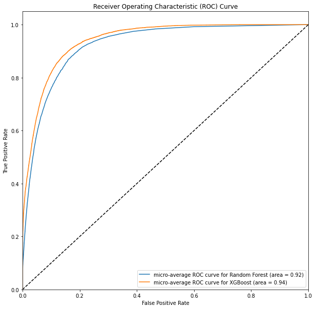
The Area Under the ROC Curve (AUC-ROC) is the evaluation metric for this project. AUC-ROC is a suitable metric when dealing with imbalanced datasets, as it considers both the true positive rate and the false positive rate, providing a robust measure of model performance across all possible classification thresholds. This characteristic makes it an appropriate choice for genre classification, where the distribution of songs across genres may be imbalanced.

Model Building Process

Data Preprocessing

The first step in the model-building process was to preprocess the data. This involved handling missing values and scaling the features. Missing values in the dataset were handled by dropping the rows with NaNs since they constituted only a small fraction of the data. In addition, columns with '?' were identified and converted to NaNs. These values were imputed with the median value of the respective column per genre.

Feature scaling was performed using the StandardScaler. This ensured that all features had a mean of 0 and a standard deviation of 1, thereby standardizing the range of the independent features in the data. Certain features such as 'instance_id', 'artist_name', 'track_name', and 'obtained_date' were dropped from the dataset because they were not significant for genre classification.

Dimensionality Reduction

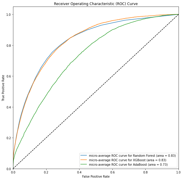
Dimensionality reduction strategies such as PCA and t-SNE were explored. However, none of these strategies improved the AUC-ROC score, indicating that these methods were not beneficial for this particular dataset.

Model Selection and Cross-Validation

The model testing process was a crucial part of the project. It began by experimenting with a variety of machine learning models on data preprocessed with t-SNE for dimensionality reduction. The models tested include Logistic Regression, Random Forest, Support Vector Machines, K-Nearest Neighbors, and XGBoost.

Logistic Regression, a simple and widely-used classification algorithm, was chosen due to its efficiency and ease of interpretation. However, it performed poorly, achieving only 0.305566 accuracy and an AUC-ROC score of 0.790516. This might be because logistic regression may not handle complex relationships in data well, particularly when there are interactions between features.

XGBoost, a powerful gradient boosting algorithm, performed better than the previous models with an accuracy of 0.471309 and an AUC-ROC score of 0.873206. The effectiveness of XGBoost can be attributed to its ability to capture complex relationships in the data and its robustness against overfitting through the use of gradient boosting.

Testing Neural Networks

Model 1 consisted of a simple feed-forward neural network with two hidden layers. The first layer had 64 neurons, and the second had 128 neurons. However, despite its simplicity, it failed to provide satisfactory accuracy.

Model 2 was a slightly larger network with more neurons in each layer (128 in the first layer and 256 in the second layer), but it also did not yield satisfactory results. This could be because while increasing the number of neurons can improve the model's capacity to learn complex patterns, it can also make it more prone to overfitting.

# Define the neural network models
class Model1(nn.Module):
    def __init__(self, input_size, num_classes):
        super(Model1, self).__init__()
        self.layer1 = nn.Linear(input_size, 64)
        self.layer2 = nn.Linear(64, 128)
        self.layer3 = nn.Linear(128, num_classes)
        
    def forward(self, x):
        x = nn.functional.relu(self.layer1(x))
        x = nn.functional.relu(self.layer2(x))
        x = self.layer3(x)
        return x

class Model2(nn.Module):
    def __init__(self, input_size, num_classes):
        super(Model2, self).__init__()
        self.layer1 = nn.Linear(input_size, 128)
        self.layer2 = nn.Linear(128, 256)
        self.layer3 = nn.Linear(256, num_classes)
        
    def forward(self, x):
        x = nn.functional.relu(self.layer1(x))
        x = nn.functional.relu(self.layer2(x))
        x = self.layer3(x)
        return x

class Model3(nn.Module):
    def __init__(self, input_size, num_classes):
        super(Model3, self).__init__()
        self.layer1 = nn.Linear(input_size, 128)
        self.layer2 = nn.Linear(128, 128)
        self.layer3 = nn.Linear(128, num_classes)
        self.dropout = nn.Dropout(0.5)
        self.batchnorm = nn.BatchNorm1d(128)
    
    def forward(self, x):
        x = nn.functional.relu(self.layer1(x))
        x = self.batchnorm(x)
        x = nn.functional.relu(self.layer2(x))
        x = self.dropout(x)
        x = self.layer3(x)
        return x

Results and Discussion

The XGBoost model achieved the best AUC-ROC score of 0.94, indicating a high performance in genre classification. The model used the original set of predictors without dimensionality reduction. This suggests that the initial feature space contained important information that was key to successful genre classification and that dimensionality reduction methods like PCA and t-SNE were unable to retain this information.

The most important features for the XGBoost classification were 'popularity', 'danceability', 'speechiness', and 'instrumentalness'. This indicates that these features have a significant impact on the genre of a song, and thus can be the focus of future research or application in similar tasks.

The final XGBoost model that was chosen uses the dataset scaled but not dimensionally reduced. This allowed the model to make use of the full feature space and achieve an AUC score of 0.94, the highest score in all the experiments. This achievement illustrates the potential of XGBoost for multi-class classification problems and encourages further exploration and application of this algorithm.